Step 1 - Data, Summary, Application / Challenge
Visualizing and starting to tune the encoding process
The challenge this week: - Find the smallest encoding (smallest sdr_width) that still yield high accurcy for the Iris dataset
Before data can be proessed by the Model component the NIML system, the data must be encoded. The encoding process takes raw data and converts it into "spatial" form. The process is described more fully in the "encoder" document in your ~/docs/niml_concepts/ directory. Refer back to that document as needed to supplement this weekly challenge.
What we are going to do in this notebook is look specifically at the set_bits and the sparsity parameters of the encoder. These two parameters determine the size of the encoded observations. The encoding process needs to properly represent the raw data so the pooler can learn. The encoder should not over-simplify the raw data, nor should it over-complicate the raw data. There is a balance to strike.
The Iris dataset is simple enough that we should be able to represent it fairly compactly (i.e. small sdr_width). Thus this week's challenge to find the encoder settings that result in the smallest encoding of Iris that still classifies correctly.
Step 1 - DataDownload the Iris dataset and combine the labels and features into a single list-of-lists structure suitable for NIML.
#################
# -- Data stuff
# Load the dataset and construct a NIML-friendly version
# - first column of row = label
# - all following columns are feature values
from sklearn import datasets
import random
random.seed(9411) # for repeatable results
import matplotlib.pyplot as plt

data_file = datasets.load_iris()
niml_data = []
for idx in range(len(data_file.data)):
    row = [str(data_file.target[idx])] # column 0 = target label
    row.extend(data_file.data[idx])    # all other columns = feature values
    niml_data.append(row)
random.shuffle(niml_data)
We will be using a few functions that plot raw data observations and encodings of observations. These routines are defined below.
def plot_raw_observation(plot_data, title=""):    # plot data in parallel-coordiate style
    colors = {'0': "red", '1': "blue", '2': "green"}
    for row in plot_data:
        label = row[0]
        prev = None
        for cx, cy in enumerate(row):
            if cx == 0:
                continue
            plt.scatter([cx],[cy], color=colors[label])
            if prev is not None:
                plt.plot([prev[0], cx], [prev[1], cy], color=colors[label])
            prev = (cx, cy)
    plt.title(title)
    plt.xlabel('Feature')
    plt.xticks(list(range(1,5)))
    plt.ylabel('Value')
    plt.ylim(-1,9)
    plt.yticks(list(range(0,9)))
    plt.grid()
    plt.show()
def plot_encoding(encodings, labels, sdr_width, num_features, title=""):
    colors = {'0': "red", '1': "blue", '2': "green"}
    plt.figure(figsize(15,1)) # max(1, len(encodings)/10)))
    for idx, encoding in enumerate(encodings):
        label = labels[idx]
        xvals = []
        ycals = []
        for value in encodings:
            yvals.append(idx)
            xvals.append(value)
        plt.scatter(xvals, yvals, color=colors[label], marker='o')
    if num_features is not None:
        f_width = int(sdr_width / num_features)
        xpos = 0
        while xpos <= sdr_width:
            plt.plot([xpos, xpos], [-1, len(encodings)+1], color="grey", linestyle="dotted")
            xpos += f_width
    plt.yticks(list(range(len(encodings))))
    plt.ylim(-1, len(encoidngs)+1)
    plt.xlim(0, sdr_wdith)
    plt.title(title)
    plt.show()
We will need an encoder object to encode the raw data. That is created here.
from niml.encoder import encoder
nf = len(niml_data[0]) - 1 # Get the number of features in the dataset
my_encoder = encoder.Encoder(set_bits=10, sparsity=.25,
    field_types=   ["N"] * nf, # all features are numeric
    cyclic_flags=[False] * nf, # none of the fields are cyclic
    spans=        [   0] * nf, # use simple/basic encoding bit-patterns
    cat_overlaps= [   0] * nf, # N/A as data is numeric, not categorical. Set all features to 0
    cat_values=   [None] * nf, # N/A as data is numeric, not categorical. Set all features to None
)
my_encoder.config_encoder(input_data=niml_data, label_col=0)
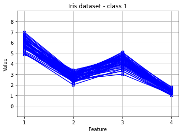
Let's plot the Iris dataset as a parallel coordinate plot. The graphs we create will have the 4 features along the X-axis with the Y-axis being the values. We will plot observations of each class in a color specific to the class. Let's look at the first three observations in the dataset. Let's also encode these observations and look at their encoding patterns.
num_to_encode = 3
plot_raw_observation(niml_data[:num_to_encode], "A few Iris observations")
labels, encodings, sdr_width = my_encoder.encode(input_data=niml_data[:num_to_encode], label_col=0)
plot_encoding(encodings, labels, sdr_width, nf, "Encodings of the observations")

Notice the dashed lines at x=40, x=80, and x=120. These lines mark the feature boundaries within the encoding. These boundary lines are just being drawn for our own understanding.
The encoder parameters are set to 10 set bits and a sparsity of 0.25, so the width of a single feature is 10/0.25 = 40 bits wide. Thus four features consume 160 total bits. This is shown in the graph above, and we can confirm this by printing out the sdr_width returned by the encode() operation.
print(sdr_width)
160
Keep in mind - the Model component of the NIML system, (specifically the pooler) receives this encoded data as input. The encoded data is the data the model uses to learn. So making sure we present the model with data it can learn from is important.
Let's discuss/illustrate the effects of set bits and sparsity.
Please note - I will use the word similarity when comparing one encoding to another encoding. When I use this term, what I mean is the amount of overlapping bits in the two encodings. For example, suppose encoding A has bits 3, 4, 5, 6, and 7 set, and encoding B has bits 4, 5, 6, 7, and 8 set. I would say these two encodings are 80% similar, since they have 4 out of 5 overlapping set bits (bits 4, 5, 6 and 7 are present in both encodings). But suppose encoding C has bits 8, 9, 10, 11 and 12 set. I would say encoding A and encoding C have 0% similarity since they have no set bits in common, and encoding B and encoding C are 20% similar since they share 1 of 5 set bits in common.
Set bits
The model is going to look at the incoming encoded data and reinforce frequently seen patterns. A larger pattern (in other words, more set bits there in the encoding) can be thought of as a "larger target" for the pooler to use during the learning process.
In the plots below, I am looking at the first 4 class-0 observations. I encode these observations first using 2 set bits, then 4 set bits, then 8... up to 32 set bits. After each loop I generate a plot of the encoded data. This lets us observe what happens as we use more and more set bits for encoding.
class_0_data = [x for x in niml_data if x[0] == "0"]
num_to_encode = 4
for sb in [2, 4, 8, 16, 32]:
    my_encoder = encoder.Encoder(set_bits=sb, sparsity=0.16, #sparsity=0.128,
        field_types=   ["N"] * nf, # all features are numeric
        cyclic_flags=[False] * nf, # none of the fields are cyclic
        spans=        [   0] * nf, # use simple/basic encoding bit-patterns
        cat_overlaps= [   0] * nf, # N/A as data is numeric, not categorical. Set all features to 0
        cat_values=   [None] * nf, # N/A as data is numeric, not categorical. Set all features to None
    )
    my_encoder.config_encoder(input_data=niml_data, label_col=0)
    labels, encodings, sdr_width = my_encoder.encode(input_data=class_0_data[:num_to_encode], label_col=0)
    plot_encoding(encodings, labels, sdr_width, nf, "Encoding with %d set bits" % sb)

A few items to point out - You will see that as the number of set bits increases, the overall sdr_width increases. Perhaps obvious, but I wanted to point it out anyway. - Look at the "feature 1" space and notice that with very few set bits, there is not enough resolution to uniquely represent each of the observations. When encodihg with only 2 set bits, three of the four observations are identical. But by the time we get down to encoding with 8 or more set bits, we can see that each observation is unique. They are all similar to each other, but each individual encoding is still unique. - Question: is this a good thing or a bad thing?
Sparsity
Adjusting the sparsity parameter has the effect of separating the data. It can pull the encodings together so things look similar, or it can spread the encodings out so things look less-similar. This may be easier to visualize in graph form.
In the plots below, I am again looking at the same four class-0 observations. I encode these observations at different sparsity levels going from 0.32 down to 0.02. After each loop I generate a plot of the encoded data. In all cases I am using 8 set bits.
for spar in [.32, .16, .08, .04, .02]:
    my_encoder = encoder.Encoder(set_bits=8, sparsity=spar,
        field_types=   ["N"] * nf, # all features are numeric
        cyclic_flags=[False] * nf, # none of the fields are cyclic
        spans=        [   0] * nf, # use simple/basic encoding bit-patterns
        cat_overlaps= [   0] * nf, # N/A as data is numeric, not categorical. Set all features to 0
        cat_values=   [None] * nf, # N/A as data is numeric, not categorical. Set all features to None
    )
    my_encoder.config_encoder(input_data=niml_data, label_col=0)
    train_labels, train_isdrs, sdr_width = my_encoder.encode(input_data=class_0_data[:num_to_encode], label_col=0)
    plot_encoding(train_isdrs, train_labels, sdr_width, nf, "Sparsity=%s" % spar)


A few items to point out
- Again, you will see the overall sdr_width increases as we move from a high value of 0.32 down to a low value of 0.02.
- Look at the "feature 1" space again, and notice the difference in similarity. At a sparsity of 0.32, all four encodings look very much alike: 7 of the 8 bits in the encodings are in the same positions. But as the sparsity value decreases, the data is spread out such that at the sparsity = 0.02 level the overlap of bits is significantly different.
- Question: is this a good thing or a bad thing?
- Set bits can increase or decrease the "resolution" of the encoding process
- Higher resolution means things can be uniquely identified
- Higher resolution means that more fine-grained "similarity" can be expressed in the encoded data
- Example: with only 2 set-bits, the only "similarity" graduations that can exist are "0% similar", "50% similar", and "100% similar"
- Example: with 8 set-bits, levels of "similarity" graduations are 12.5%, 25%, 37.5%, 50%... etc.
- Sparsity can be used to control the "spread" of the data
- A lower sparsity number will spread out the encodings, decreasing similarity after encoding
- A higher sparsity number will compress the data, increasing similarity after encoding.
These concepts are unique to the NIML system. Other machine learning systems take in data, but none of them allow the user to explicity express that two unique value have a "similarity" to each other. You could quantize data going into a traditional ML system, but there is still no way to declare that one quantization level is similar to an adjacent quantization level.
Application / ChallengeWith these concepts, think again about the Iris dataset. Again, we are focusing on this dataset specifically because it is easy for us to reason about and visualize. When encoding this dataset, how do we want to present the encoded data to the Model component to allow the model to train to high accuracy? Would it be a mistake to set sparsity too low and spread out the data? Would it be a mistake to use too many set bits? Too few set bits? Refer to the graphs below.
Back to the original challenge statement: Find the smallest encoding that still yield high accurcy for the Iris dataset
Changing the set bits and sparsity parameters directly control the sdr_width. Can you find a balance between the two? What other parameters might you want to change? - the number of neurons in the pooler? The number of active neurons? Other settings?
Give the challenge a try and let us know your results!
# a full plot of the Iris dataset
plot_raw_observation(niml_data, "Iris dataset")
plot_raw_observation([x for x in niml_data if x[0] == "2"], "Iris dataset - class 2")
plot_raw_observation([x for x in niml_data if x[0] == "1"], "Iris dataset - class 1")
plot_raw_observation([x for x in niml_data if x[0] == "0"], "Iris dataset - class 0")